Planning and Managing Distance Education Systems: Building the Model
Dr. Fred Saba
Farhad Saba, Ph. D.
Founder and Editor, Distance-Educator.com
In this series of articles, I presented a hierarchical model of distance education consisting of seven interrelated nested systems levels. These systems have been present in most distance education organizations that I observed, or planned and built over the past 30 years. In the previous weeks, I discussed Hardware, Software, Telecommunications, Instructional, Educational, Societal and Global Systems Levels. Last week I started to explain the process of system modeling so that you could start the planning process for your organization. I hope that conducting the environmental scan as presented in a previous article has given you a better appreciation of the components of the technology-based educational programs in your organization and the interrelationships among such components. But before I went any further on the process of modeling itself, I explained certain important concepts in system methodology in this article and showed how these principles can be applied in this article titled Planning and Managing Distance Education Systems: Applying system dynamics. Below, you will see an example in systems modeling in detail.
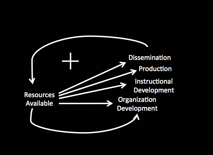
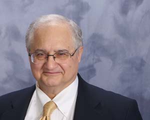
Figure 1- Causal loop diagram of a simple model of a distance education system adapted from Saba, and Twitchell 1988.
In Figure 1, the more resources that are available to an organization the more funds are available for its four essential activities, namely organization and instructional development, as well as production and dissemination. In other words, decisions that lead in making more funds available by organization development, instructional development, production and dissemination would provide additional funds available—a positive feedback loop. Further, such relationships are simple in mathematical terms, as they are signified by a (+) sign in the diagram indicating that more resources leads to more activities in the four related components. The terminology used in building the diagram is common in the fields of educational technology and distance education, and the diagram can be extended to include many more components as the planning process may need it. For example, external components in the form of government policies that can increase or decrease resources available to the system can easily be added to the diagram. The loop can also accommodate continuous interactions, although delays in decisions or certain functions may occur. In other words, there would always be a time delay between providing funds for a function, such as, instructional design, and the time that the design documents for the each course would be ready for the use of the production crew to make the television programs.
Formulating acceptable formal decision policies that describe how decisions result from the available information streams.
The purpose of the simulation study was twofold: First it was to find out if the initial number o f students enrolled in a distance education system affected the resources allocated to the system? In other words, were there an optimal number of students necessary to generate enough income in a distance education system to make it viable in the long run? Second, the study was to determine how resources available to a system affected the performance of each system component? Put differently, the study focused on resources available to an organization that can be spent on organizational and instructional development, production of instructional materials and dissemination of courses to support a certain number of enrollments. Dissemination of courses in the model led to enrollments as well as graduates and dropouts. At each point in time student population depended on the number of enrollments minus those that have graduated or dropped out. At each point in time student population determined the resources available to the system at which point the causal loop repeats itself. This model was run several times based on different assumptions in terms of initial dollar amounts of resources available in order to determine the level of student population which would make the system sustainable relative to its income from dissemination of courses. Undoubtedly distance education systems in operation in colleges and universities are more complex than this model. However, as an initial study in 1988, the objective was to define the boundary of the system so that it would include a small but sufficient number of components. As it turned out, even this small model had to be expanded a bit to make it operational on a computer, as it is evident in the flow diagram of the system.
Construct a mathematical model of the decision policies, information sources, and interactions of the system components.
Defining Relations– Relations among components in a system are governed by two kinds of feedback loops: positive and negative. Figure 2 shows an example of a positive feedback loop in which it is indicated that the more resources available, the more can be spent on organization development.
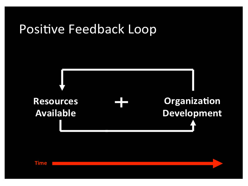
Figure 2- Example of a Positive Feedback Loop
Negative feedback loops indicate that the more the value of a component increases the less of another component is available in a system.
Figure 3- Example of a Negative Feedback Loop
Negative feedback loops provide control in a system. As shown in Figure 3 the more students graduate the less the level of student population would be. The control process in this loop includes another component of the system that of enrollments in the sense that the lower the student population, the more room there is for enrolling new students. A classic example of a negative feedback loop as a control mechanism is the home thermostat. As the temperature in a house decreases, the thermostat element is contracted to make a connection, which in turn starts the furnace. As the temperature increases, the thermostat element is expanded and disconnected. As the result the furnace shuts down.
Figure 3. Example of a negative and a positive feedback loop as a control mechanism
There is no, inherent value to these loops. A “positive” loop is no better or worse than a “negative” one; they have different functions and play specific roles in various circumstances. Most living systems and organizations are complex, and many positive and negative loops define the relationships among their various components.
Developing a Flow Diagram– In this step in the modeling process, a flow diagram was developed based on the causal loop diagram. The purpose here was to visualize the relations among system components in in terms of decisions that influenced the behavior of each of the systems components and the entire model as a whole. The flow diagram also assisted in writing the system equations that would represent the model in mathematical terms. The flow diagram as presented in Saba, and Twitchell (1988) is presented below as an example, followed by a prose description of it.
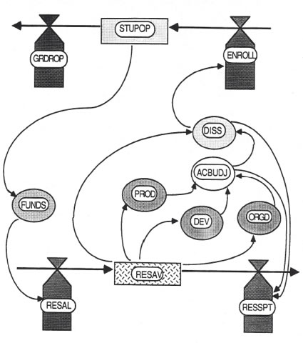
Figure 4- Flow diagram of a simple distance education system
Figure 4- Flow diagram of a simple distance education system
“The level of available resources to a distance education system at the present time (RESAV.K) is assumed to be affected by a steady rate of monetary allocations (RESAL) from funds that are dependent upon the number of students enrolled. The rate of expenditure (RESSPT) is increased or decreased by four functions or auxiliaries: organization development (ORGD), instructional development (DEV), and production of instructional materials (PROD). It is assumed that these auxiliaries control the rate of a fourth auxiliary, which is dissemination (DISS). Dissemination in turn controls the rate of enrollments (ENROLL) and the rate of enrollments affects the level of student population at the present time (STPOP.K). In addition, this level is affected by another rate which reflects the students who graduate or drop out of the system. Student population at the present time influences an auxiliary for funds, which in turn controls the rate of resources allocated to the system.” (pp. 16).
System Equations– As mentioned above, the two primary building blocks of system dynamic models are stocks (levels) and rates. In the following an example of an equation for each of these primary components are presented. The equation for the stock resources available at each point in time. As Forrester put “A good test to determine whether a variable is a level or a rate is to consider whether or not the variable would continue exist and to have meaning in a system that had been brought to rest.” (Forrester 1961 Page 68). In this model, if enrollments continue at a steady rate the level of student body would remain at a certain number provided that that the rate of graduation and dropouts equals the rate of enrollments. Rates, on the other hand, represent decisions. In other words, the rate at which funds become available for each of the four system functions is a decision that is made by the manager of a distance education organization or a similar authority. This decision can be changed in different iterations of the simulation to see how it would affect the performance of each component and the system in its entirety. A prose description of the equations is presented below.
RESAV.K=RESAV.J+(DT)(RESAL.JK-RESSPT.JK)
In prose language the above equation means resources available at this point in time equals resources available at one time interval before the present time, plus the interval elapsed multiplied by resources allocated in that time interval, minus resources spent in that time interval.
An example of a rate equation is as follows:
REASAL.KL=FUNDS.K/T
In prose language the above equation means, resources allocated during a time interval equals the amount of funds divided by the time interval elapsed.
There are other types of equations necessary to simulate the model above such as those that define auxiliaries. However, we will confine our discussion of developing equations only to these two types of primary components in a model at this time.
The important point to consider in the process of model building is focusing on the development of the flow diagram and making sure that it represents the operation of your organization as best as those who are involved in it can depict. Therefore, model building in most organizations requires the participation of those who are in charge of the operation of each component on a day-today basis. Ultimately, any change in the organization as the result of your planning process must be administered by them. It is important that the members of the organization ranging from students to faculty, administrators, etc. be involved in the model building process as much as possible, and agree on the fidelity of the model in representing what they do.
Generate the behavior through time of the system as described by the model (usually with a digital computer to execute the lengthy calculations) In this example the model was run on an Apple II computer using DYNAMO (DYNAmic MOdels) software which was major improvement in the time and effort needed to complete task as compared to using system dynamic compilers on main frame computers. What used to take weeks to accomplish, was now possible to do in a matter hours if not minutes! The side bar here presents a quick overview of the evolution of simulation technology in recent years
| Simulation technologyWith the advent of the mainframe computer, it became possible to process considerable amount of data about components and operations of different types of organizations ranging form factories, and oil refineries, to banks and schools. In addition, simulation software allowed for assessing how components that constitute different systems in organizations relate to each other and behave over a period of time.
As computers became more efficient and less expensive, researchers, planners, managers and decision makers were enabled to conduct simulations on microcomputers. System Dynamics, the modeling and simulation method used in this book, was such a simulation technology which in the 1960s and 70s was available on the main frame computers. By the 1980s, it also became available as DYNAMO (DYNAmic MOdels) on the Apple II computer, and then as STELLA (Structural Thinking Experimental Learning Laboratory with Animation) on the Macintosh and the PC. Developed by isee systems, STELLA offers a graphical user interface to simulate system models in education widely. (http://www.iseesystems.com/). STELLA is not the only software technology with which system dynamics model building is possible. Vensim is another example of a powerful tool for this purpose (http://vensim.com/). However, the authors of this book have used STELLA over the years in their research, development and teaching and the models presented in this book were built on Apple computers either using DYNAMO or STELLA. |
Compare results against all pertinent available knowledge about the actual system.
The model building effort in this case was in response to Hawkridge and Robinson’s recommendations that
a) Managers should carry out detailed analyses of financing for educational broadcasting and, to avoid neglecting potential resources, and
b) In the same way they should carry out analyses based on functions of (for example general administration, conception, production, distribution, utilization, evaluation) to enable them to determine the balance of resources allocated to each function and whether this is the correct balance (pp. 149-150).
To assess the model in relation to the above policy considerations and related decisions, several runs were made to test the equations and debug the formulas. Then the model was run under two different initial enrollment levels. The first run of the model represented a student population of 75 out of a total potential student population of 500 (or 15%). Under this condition in a 48 month period the following changes in the behavior of the model were observed
- the level of resources available to the system declined and continued to decrease, while the level of student population increased moderately (slightly surpassing 100) and then started to level off. (See Plot No. 1.1.)
- There was a dramatic decline in the rate of enrollments in the first six months of the operation. The decline was not as dramatic after this period, but it did continue to do so. The rate of graduation slowly increased in the first year and then it slowed down to approach the same value as the rate of enrollments.
- The functions also declined throughout the time of the simulation. The most dramatic was the rate of production which showed a steady decline throughout the 48 months. All other functions, instructional development, organization development and dissemination also declined toward zero.
Revise the model until it is acceptable as a representation of the actual system.
For the second run of the model the initial student population was changed to 100 to represent 20% of the total possible population. Under this condition it was observed that:
- The level of available resources declined slightly in the first few months, but then it went back to its initial value and stayed there for the rest of the time. The level of student population, however, showed a dramatic increase to almost include the total potential population near the 48th month.
- The rate of enrollments showed a decline during the first two years of the operation, while the rate of graduation increased during this time. As it could be expected, both rates showed a tendency to approach the same value in the future.
- The rate of resources allocated decreased slightly in the first half of the simulation, but then the rate went back to its initial value, and remained there. Whereas, the rate of expenditure showed a dramatic increase during the first 18 months, and although it began to slow down, it still remained at an impressive value.
- The rate of functions experienced healthy values in this run. Production declined slightly during the first half of the simulation time, then it increased to regain its initial value. Instructional development, organizational development, and dissemination, however, kept the same rate of performance during the entire time.
Redesign, within the model, the organizational relationships and policies which can be altered in the actual system to find the changes which improve system behavior.
This model had no real referent. It was primarily built to test the application of system dynamics to modeling distance education operations, based on aggregate information distilled from the study of 12 different educational television institutions. However, the results clearly indicated that a 10% initial rate of enrollments is inadequate to sustain the system for an appreciable amount of time. Enrollments must be at 20% to make the operation sustainable. These results are useful for new programs within well established universities so that policy makers can have a more realistic expectation of how the project may mature and bear fruit. The results, however, are critical for start-up for profit institutions that must perform at a certain level before their operations fall to a pattern of behavior that would drag the enterprise to a certain death.
Alter the real system in the directions that model experimentation has shown will lead to improved performance.
In the absence of a real referent organization, we were not able to make any changes to the structure and operations of such an organization towards the direction that the model suggested to see if the desired and expected results would have materialized. However, this is an important aspect of the modeling process for your organization as this is where you would realize the fruits of the planning and modeling effort to move the organization forward towards further development. If this model building exercise was based on a real organization, the results would have been of crucial value at least for the marketing and enrollment operations, as the number of enrollments proved to be very important in the future well being of the system.